firas midani

Primer on modelling bacterial growth: Why do we log-transform optical density?

11 July 2019

Bacteria replicate by binary fission: each bacterial cell splits into two daughter cells, who go on to split to form four cells, who split to form eight cells, and so on. Accordingly, a bacterial community grows by doubling at each generation. This can be mathematically expressed as follows:

\begin{equation} N(i+1) = N(i) \times 2 \end{equation}

where $i$ indicates generation number and $N(i)$ indicates population size at generation $i$. We can further simplify population size, with a closed-form solution, as a function of the initial population size $N(0)$, number of generations $i$, and growth factor $g$.

\begin{equation} N(i) = N(0) \times g^i \end{equation}

Because we are modelling bacterial growth, we will simply assume that bacteria always replicate by doubling and therefore growth factor $g$ must equal $2$.

\begin{equation} N(i) = N(0) \times 2^i \end{equation}

The most common method for measuring bacterial growth is spectrophotometry, where the absorbance or optical density (OD) of a bacterial culture is proportional to population size¹ and absorbance is measured over time. Therefore, we can model absorbance as a function of microbial population size.

\begin{equation} A(t) \propto N(i) \end{equation}

Because we are interested in modelling the absorbance as a function of time, we need to properly substitute the $i$ exponent (number of generations) with a corresponding function of time.

\begin{equation} n = \frac{t}{\tau} \end{equation}

where $\tau$ is the generation time, i.e., how long it takes for a new generation to arise or, in the specific case of bacteria, how long it takes a parent cell to split into two daughter cells. This yields the following estimate of absorbance as a function of time

\begin{equation} A(t) = A(0) \times 2^{t/ \tau} \end{equation}

By measuring absorbance at multiple intervals of time, we can capture a bacterial growth curve and we are primarily interested in capturing the maximum growth rate of the population during exponential growth phase. The derivative of our growth curve (i.e. absorbance) at time $t$ when bacteria are growing fastest (curve is steepest), should give us the maximum population growth rate.

\begin{equation} \frac{d}{dt}A(t) = \frac{d}{dt}\left[A(0)\times 2^{t/\tau}\right] = A(0)\times \frac{1}{\tau} \times \ln{2} \times 2^{t/\tau} \propto2^{t/\tau} \end{equation}

Here, we see that the derivative remains (i) an exponential function of time (i.e. time is variable in the exponent) and (ii) derivative of absorbance is proportional to itself (Equation 7). These are two intrinsic property of exponential functions.

Per Wikipedia page on Exponential Function,

As functions of a real variable, exponential functions are uniquely characterized by the fact that the growth rate of such a function (that is, its derivative) is directly proportional to the value of the function. The constant of proportionality of this relationship is the natural logarithm of the base b: $\frac{d}{dx}b^x = b^x \log_{e}b$

However, we want an estimate of growth rate that is proportional or independent of time (i.e., not exponential to time). To overcome this issue, we can take advantage of a useful mathematical property of exponential functions. If a “variable exhibits exponential growth, then the log (to any base) of the variable grows linearly over time” as I demonstrate below. Recall that

\begin{equation} A(t) = A(0) \times 2^{t/ \tau} \end{equation}

and that $\log_{b}{(x^d)}=d\log_{b}{(x)}$ such that

\begin{equation}\ln{A(t)} = \ln{\left(A(0)\times2^{t/ \tau}\right)}\end{equation} \begin{equation}\ln{A(t)} = \ln{A(0)} + \ln{(2^{t/ \tau})}\end{equation} \begin{equation}\ln{A(t)} = \ln{A(0)} + \frac{t}{\tau}\ln(2)\end{equation} \begin{equation}\ln{A(t)} = \ln{A(0)} + \left(\frac{\ln{2}}{\tau}\right)t\end{equation}

We can easily take the derivative of the natural logarithm of $A(t)$

\begin{equation}\frac{d}{dt}\ln{A(t)} = \frac{d}{dt}\ln{A(0)} + \frac{d}{dt}\left(\frac{\ln{2}}{\tau}\right)t\end{equation} \begin{equation}\frac{d}{dt}\ln{A(t)} = \left(\frac{\ln{2}}{\tau}\right)\end{equation}

As you can see the natural logarithm of absorbance is now a function of time $t$ (Equation 12) . This relationship is akin to the didactically classical form of a linear function $y=b+mx$ from basic algebra, where $y$ is the dependent variable, $x$ is the independent variable, $b$ is the y-intercept, and $m$ is the slope.

\begin{equation} m = \frac{d}{dt}\ln{A(t)} = \left(\frac{\ln{2}}{\tau}\right) \end{equation}

We refer to $m$ as the maximum specific growth rate² . Because we assumed that growth factor is two (i.e., bacteria reproduce by doubling), the inside of the natural logarithm is two (the base of exponent in Equations 3 and 8). Further, once we estimate the maximum specific growth rate, we can easily compute doubling time as

\begin{equation} \tau = \left(\frac{\ln2}{m}\right) \end{equation}

We could have taken the natural logarithm of Equation 8 to any base that is larger than 1 and assumed a growth factor different than two. Eventually, we would always end up with the following generalized expression

\begin{equation} \tau = \left(\frac{\log_{b}{g}}{m}\right) \end{equation}

where $b$ is the base of the logarithm used for simplifying the model, $g$ is the growth factor, and $m$ is the maximum specific growth rate. The $e=2.71828$ constant (base of natural logarithm) is often used because it has interesting mathematical properties. For example, it is the “unique base for which the constant of proportionality is 1, so that the exponential function’s derivative is itself” $\frac{d}{dt}e^{t}=e^{t}\log_{e}{e}=e^{t}$. Still, any other base larger than 1 can be used. Data should be transformed with the logarithm of the selected base, maximum specific growth rate can then be computed, and doubling time inferred from Equation 17.

In the case of non-parametric Gaussian Process Regression of growth curve data, the maximum a posteriori (MAP) estimate of the derivative of the logarithm-transformed is $m$. Growth curves analyzed with classical models (e.g., logistic or gompertz) directly capture a parameter that corresponds to the maximum specific growth rate, often referred to as $r$ which is also assumed to be the slope of growth during exponential phase. These models inherently account for exponential growth by including $e^{-rt}$ in their mathematical expression,

\begin{equation} A(t) = \frac{K}{1+\left(\frac{K-N(0)}{N(0)}\right)e^{-rt}} \end{equation}

such that doubling time can be computed with Equation 16 directly with the estimate of $r$ or $m$; in these cases, because the base is $e$, the numerator for $\tau$ is the natural logarithm of two.

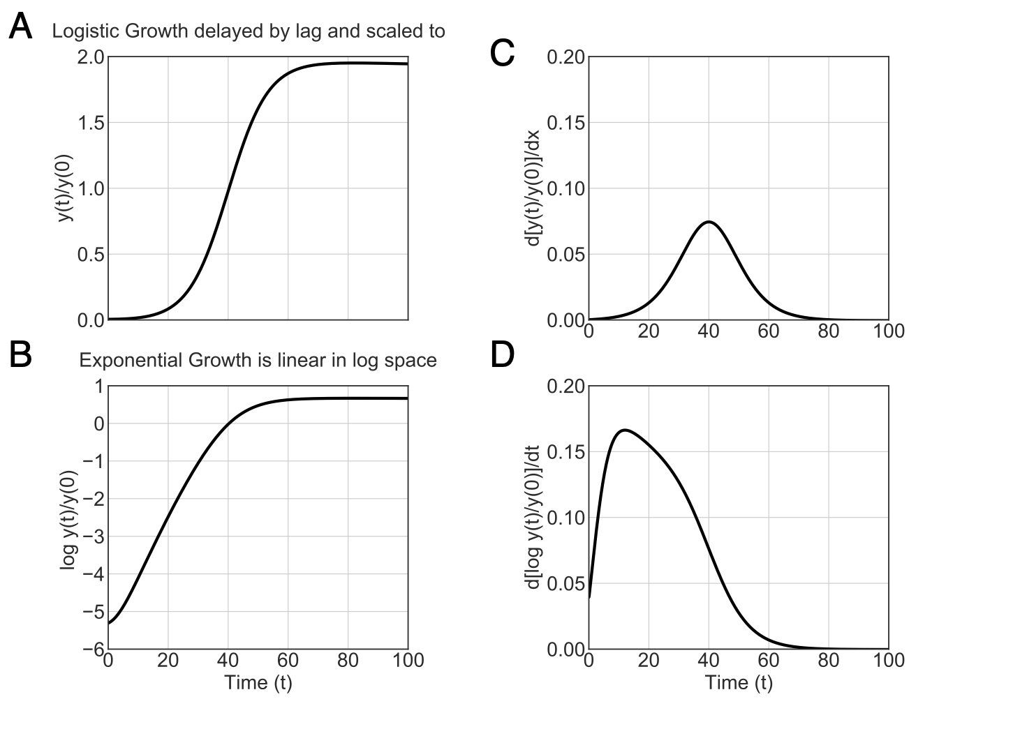
Below is a simple example comparing the classical and GP-based models. I simulated logistic growth superimposed with a linear negative delay (Figure 1A). As expected, there is a slight lag followed by exponential growth that starts to slow down leading to linear increase in OD around $t=40$ eventually plateauing at $y=2$. The logarithm transformation of $y(t)$ shows the exponential growth as linear growth in log-space (Figure 1B). The derivative of untransformed $y(t)$ captures the maximum linear phase of growth which occurs after the population exits exponential growth (Figure 1C). However, the derivative of the logarithm-transformed $y(t)$ captures the maximum specific growth rate (during exponential growth) as $~0.16$ (Figure 1D). The true growth rate in the logistic model (Equation 18) was set to $0.15$.