Example Pipeline
Table of Contents
- Hypothetical scenario
- Preparing your data for analysis
- Plotting growth curves
- Fitting growth curves
- Normalizing growth parameters
- Plotting heatmaps
- Simple Hypothesis Testing
To follow along with this example, you will find the necessary files in the amiga/example git folder.
Hypothetical scenario
You are the leading global expert on the human pathogen Examploides randomii. Diligent work by your lab has previously analyzed its outbreak in the United States of America (USA) in 1995. One week ago, you received a phone call from Mariana, an epidemiologist in Mexico (MEX). E. randomii is emerging in the the state of Yucatán. Mariana has been tracking the outbreak and is wondering if the emerging strain may be related to the 1995 outbreak in USA. She has sent you two clinical isolates of E. randomii overnight. You revived two clinical isolates from frozen stocks of the 1995 outbreak. You asked your colleague, Kai, to sequence and compare the genomes of all of the isolate. In the meantime, you profiled the carbon substrate utilization of all isolates using Biolog Phenotype Microarray (PM) plates 1 and 2.
Preparing your data for analysis
You created a working directory in /home/outbreaks/erandomii and saved the result from your plate reader in /home/outbreaks/erandomii/data.
You also created the following table describing your files and saved it as the tab-delimited mapping file /home/outbreaks/erandomii/mapping/meta.txt
| Plate_ID | Species | Strain | Isolate | PM | Replicate |
|---|---|---|---|---|---|
| ER1_PM1-1 | E_randomii | USA_1995 | ER1 | 1 | 1 |
| ER1_PM1-2 | E_randomii | USA_1995 | ER1 | 1 | 2 |
| ER1_PM2-1 | E_randomii | USA_1995 | ER1 | 2 | 1 |
| ER1_PM2-2 | E_randomii | USA_1995 | ER1 | 2 | 2 |
| ER2_PM1-1 | E_randomii | USA_1995 | ER2 | 1 | 1 |
| ER2_PM1-2 | E_randomii | USA_1995 | ER2 | 1 | 2 |
| ER2_PM2-1 | E_randomii | USA_1995 | ER2 | 2 | 1 |
| ER2_PM2-2 | E_randomii | USA_1995 | ER2 | 2 | 2 |
| ER3_PM1-1 | E_randomii | MEX_2020 | ER3 | 1 | 1 |
| ER3_PM1-2 | E_randomii | MEX_2020 | ER3 | 1 | 2 |
| ER3_PM2-1 | E_randomii | MEX_2020 | ER3 | 2 | 1 |
| ER3_PM2-2 | E_randomii | MEX_2020 | ER3 | 2 | 2 |
| ER4_PM1-1 | E_randomii | MEX_2020 | ER4 | 1 | 1 |
| ER4_PM1-2 | E_randomii | MEX_2020 | ER4 | 1 | 2 |
| ER4_PM2-1 | E_randomii | MEX_2020 | ER4 | 2 | 1 |
| ER4_PM2-2 | E_randomii | MEX_2020 | ER4 | 2 | 2 |
Plotting growth curves
You are curious about the quality of your results. Is the pathogen growing in at least some of the wells? Is the data noisy? Do you need to repeat any plates?
You downloaded AMiGA (see Installation) and made sure you are in the correct directory.
cd /home/programs/amiga
You started analyzing your data by simply plotting the files.
amiga summarize -i /home/outbreaks/erandomii/
You found the following files in your figures folders:
ER1_PM1-1.pdf
ER1_PM1-2.pdf
ER1_PM2-1.pdf
ER1_PM2-2.pdf
ER2_PM1-1.pdf
ER2_PM1-2.pdf
ER2_PM2-1.pdf
ER2_PM2-2.pdf
ER3_PM1-1.pdf
ER3_PM1-2.pdf
ER3_PM2-1.pdf
ER3_PM2-2.pdf
ER4_PM1-1.pdf
ER4_PM1-2.pdf
ER4_PM2-1.pdf
ER4_PM2-2.pdf
and the following file sin your summary folders:
ER1_PM1-1.txt
ER1_PM1-2.txt
ER1_PM2-1.txt
ER1_PM2-2.txt
ER2_PM1-1.txt
ER2_PM1-2.txt
ER2_PM2-1.txt
ER2_PM2-2.txt
ER3_PM1-1.txt
ER3_PM1-2.txt
ER3_PM2-1.txt
ER3_PM2-2.txt
ER4_PM1-1.txt
ER4_PM1-2.txt
ER4_PM2-1.txt
ER4_PM2-2.txt
Gladly, all figures look fine. The pathogen seems to be growing in some of the wells in each of the PM1 and PM2 plates. There are some minor difference that you can spot by eye between the Mexican and American isolates. But you will fit the growth curves first to confirm your observations.
Fitting growth curves
To fit the growth curves, you run the following command. The --merge-summary argument will report the results in a single text file with the name passed with the -o argument Biolog_ERandomii. Fitting growth curves takes about 1 minute per 96-well plate. The full analysis will take about 15 minutes. You added the --verbose argument so that AMiGA shares in real time more details about the input, data processing, and results.
amiga fit -i /home/outbreaks/erandomii --merge-summary -o "Biolog_ERandomii" --verbose
Normalizing growth parameters
New files in your summary folder with the summary suffix were created and include inferred growth parameters for each well. Next, you normalized all of the growth parameters relative to the relevant control well (A1 in Biolog plates) shown below.
amiga normalize -i /home/outbreaks/erandomii/summary/Biolog_ERandomii_summary.txt --normalize-method "division" --group-by "Plate_ID" --normalize-by "Substrate:Negative Control" --verbose
Plotting heatmaps
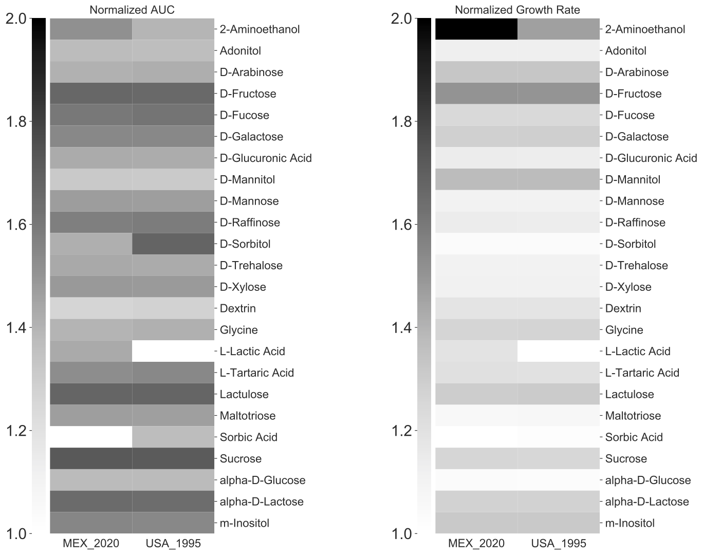
Next, you can look at these results in your favorite data analysis software (e.g. Python, R, Microsoft Excel). You wanted to plot heatmaps for parameters but only include substrates with normalized AUC higher than 1.2. You can filter the data manually or your using software and then pass the summary file to the heatmap function or you can do it some basic filtering internally with the heatmap function. Here is how to do this with AMiGA.
amiga heatmap -i /home/outbreaks/erandomii/summary/Biolog_ERandomii_summary_normalized.txt -o Biolog_ERandomii_summary_norm_auc --verbose -x Strain -y Substrate -v "norm(auc_log)" -p "mean" --filter "row any > 1.2" --kwargs "cmap:Greys;vmin:1;vmax:2" --title "Normalized Growth AUC" --save-filtered-table
amiga heatmap -i /home/outbreaks/erandomii/summary/Biolog_ERandomii_summary_norm_auc_filtered.txt -o Biolog_ERandomii_summary_norm_gr --verbose -x Strain -y Substrate -v "norm(gr)" -p "mean" --kwargs "cmap:Greys;vmin:1;vmax:2" --title "Normalized Growth Rate"

You made the following observations:
- Only the MEX_2020 strain grows on L-Lactic Acid.
- Only the USA_1995 strain grow on Sorbic Acid..
- MEX_2020 strain seems to grow much better on 2-Aminoethanol.
- USA_1995 strain seems to grow much better on D-Sorbitol.
- MEX_2020 strain seems to grow more rapidly on 2-Aminoethanol than USA_1995.
- Capric Acid is toxic to both strains.
Simple Hypothesis Testing
Based on your observations, you formulated several hypothesis. You can test for those quickly with AMiGA. For example, you tested for differential growth on L-Lactic Acid between the two strains using the following command.
amiga test -i /home/outbreaks/erandomii -s "Substrate:L-Lactic Acid" -y "H0:Time;H1:Time+Strain" -o "strain_difference_l_lactic_acid" -np 99 -tss 3 --subtract-control --verbose
This will produce six files in the strain_difference_l_lactic_acid folder inside the models directory:
strain_difference_lactic_acid_key.txtstrain_difference_lactic_acid_input.txtstrain_difference_lactic_acid_params.txtstrain_difference_lactic_acid_log.txtstrain_difference_lactic_acid_report.txtstrain_difference_lactic_acid.pdf
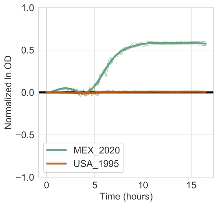
The figure will show the models estimated for each strain (bold lines) overlaid on the actual data (thin lines). Shaded bands indicate the 95% confidence interval for the models.

The output report will look like this:
The following criteria were used to subset data:
Substrate......['L-Lactic Acid']

The following hypothesis was tested on the data:
{'H0': ['Time'], 'H1': ['Time', 'Strain']}

log Bayes Factor = 666.990 (0.0-percentile in null distribution based on 100 permutations)

For P(H1|D) > P(H0|D) and FDR <= 10%, log BF must be > 0.937
For P(H0|D) > P(H1|D) and FDR <= 10%, log BF must be < -0.000

The functional difference [95% CI] is 4.300 [4.119,4.481]

Data Manipulation: Input was reduced to 34 equidistant time points. Samples were normalized to their respective control samples before analysis.
This indicates that the log Bayes Factor is 666.990 and much higher than the 10% FDR threshold of 0.937. You are every confident that Lactic Acid supports the growth of the MEX_2020 strain but not the USA_1995 strain.
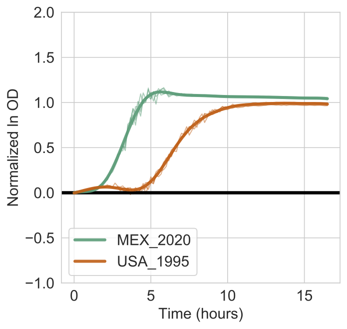
For an additional illustration of this approach, you tested for differential growth of these strains on 2-Aminoethanol using the following command:
amiga test -i /home/outbreaks/erandomii -s "Substrate:2-Aminoethanol" -y "H0:Time;H1:Time+Strain" -o "strain_difference_2_aminoethanol" -np 99 -tss 3 --subtract-control --verbose
The log Bayes Factor was 542.706 and much higher than the 10% FDR threshold of 0.502. You are also confident that the MEX_2020 strain has a faster growth rate on 2-aminoethanol than the USA_1995 strain.

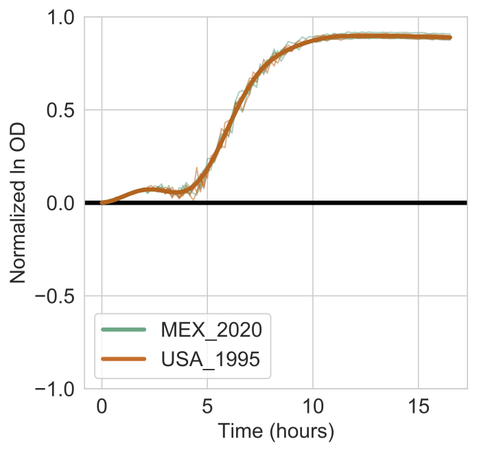
As a control, you tested for differential growth on D-Xylose. The above heatmap suggests that there is very little difference in AUC or growth rate between the strains.

There is almost no visual difference of the strain-specific models. The report also shows that the log Bayes Factor is 0 and that the 10% FDR threshold is 0.087. Recall, that git \(\text{Bayes Factor} = \exp{\log \text{Bayes Factor}} = \exp{0} = 1\)
and
\[\text{Bayes Factor} = \frac{P(H1|D)}{P(H0|D)}\]Therefore, the analysis suggest that alternative hypothesis that strain differences contributes to differences in growth is not more informative than the null hypothesis that only time explains variations in optical density measurements at an FDR set to 10%.